Identifying sources
phoptic uses photutils to find sources in images. This notebook will demonstrate how to define source finders for use with phoptic, as well as explain phoptic’s default behaviour when no source finder is specified.
Test Image
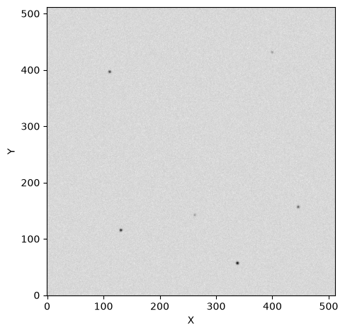
First thing’s first, let’s open an image that contains some sources. For this example, I’ll use one of the images from the Basic Usage tutorial:
[1]:
from pathlib import Path

import phoptic

out_dir = Path('out')

phoptic.generate_observations(
    out_directory=out_dir / 'data',
    n_images=3,
    circular_aperture=False,
    )
[OPTICAM] variable source is at (131, 115)
[OPTICAM] variability RMS: 0.02 %
[OPTICAM] variability frequency: 0.135 Hz
[OPTICAM] variability phase lags:
    [OPTICAM] g-band: 0.000 radians
    [OPTICAM] r-band: 1.571 radians
    [OPTICAM] i-band: 3.142 radians
Generating observations: 100%|████████████████████████████████████████████████████████████████████████████████████████████████████████████████████████████████████|[00:00<00:00]
[2]:
from astropy.io import fits
import numpy as np
import os

files = os.listdir(out_dir / 'data')
file = files[0]

with fits.open(out_dir / 'data' / file) as hdul:
    print(repr(hdul[0].header))
    image = np.array(hdul[0].data)
    binning_factor = int(hdul[0].header['BINNING'][0])
SIMPLE  =                    T / conforms to FITS standard
BITPIX  =                  -64 / array data type
NAXIS   =                    2 / number of array dimensions
NAXIS1  =                  512
NAXIS2  =                  512
EXTEND  =                    T
FILTER  = 'i       '
BINNING = '4x4     '
GAIN    =                  1.0
EXPOSURE=                  1.0
DARKCURR=                  0.0
INSTRUME= 'OPTICAM '
AIRMASS =                    1
RA      =                  0.0
DEC     =                  0.0
UT      = '2024-01-01 00:00:01'
[3]:
from astropy.visualization import simple_norm
from matplotlib import pyplot as plt

fig, ax = plt.subplots(tight_layout=True)

im = ax.imshow(
    image,
    norm=simple_norm(image, stretch="sqrt"),
    origin="lower",
    cmap="Greys",
    )

ax.set_xlabel("X")
ax.set_ylabel("Y")

plt.show()
Default Finder
phoptic implements two default source finders: Finder (default) and CrowdedFinder (better for crowded fields, but more expensive). Finder does not implement any source deblending, while CrowdedFinder does. Both of these source finders are wrappers for photutils.segmentation.SourceFinder with some added convenience tailored to OPTICAM.
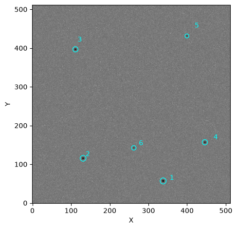
Let’s use phoptic.Finder to identify the sources in the above image:
[4]:
from phoptic import DefaultFinder

from photutils.segmentation import detect_threshold

# default value for n_pixels is 128 // binning_factor**2
# default value for border_width is 1/16th of the image width
default_finder = DefaultFinder(n_pixels=128 // 4**2, border_width=image.shape[0] // 16)

default_tbl = default_finder(
    image,
    threshold=detect_threshold(image, n_sigma=5),  # 5 sigma detection threshold
    )
print(type(default_tbl))
default_tbl.pprint_all()
<class 'photutils.utils._deprecation.DeprecatedColumnQTable'>
label     x_centroid         y_centroid     sky_centroid bbox_xmin bbox_xmax bbox_ymin bbox_ymax area   semimajor_axis     semiminor_axis      orientation         eccentricity        min_value          max_value         segment_flux    segment_flux_err     kron_flux      kron_flux_err
                                                                                                 pix2        pix                pix                deg
----- ------------------ ------------------ ------------ --------- --------- --------- --------- ---- ------------------ ------------------ ------------------ ------------------- ------------------ ------------------ ------------------ ---------------- ------------------ -------------
    1  338.0825312058613  56.89820802899701         None       335       341        54        60 39.0 1.5632332553138488 1.4575955813065393 317.47165450299735  0.3613671651919591 150.84585894595648  706.2777407047554 12064.268946598944              nan  57639.52286021281           nan
    2 131.04789276069786 115.28043522412558         None       128       134       112       118 33.0  1.504927321270826 1.3801342976383668  48.05087242396253 0.39871004163807827 152.68171418033708  566.4609974581167  9297.974211130544              nan  54290.58863127251           nan
    3  111.2627533431767 396.74739953989837         None       109       114       394       399 27.0 1.3584564292339647 1.3049155353306825  48.71347707909958 0.27797965226442944 152.50612259832968  469.8003730388308  7353.119679256409              nan  46554.66987069718           nan
    4 445.86794437886306 156.73585721659478         None       443       448       154       159 24.0 1.3652509419512628 1.2370485148077872 306.98276728653053  0.4230719910586666  150.9910429351179  397.6897729914111  5711.569358403683              nan  45648.91831303492           nan
    5 399.51375862939966 431.29897605996086         None       398       401       430       433 14.0 1.0368200711438733  1.021302380225006  323.3336125258134  0.1723636800676426 163.22942799156786  222.0908781875106  2551.929493305932              nan  30680.41446239951           nan
    6 262.14435252861097 142.30912925040474         None       260       264       141       144 12.0 1.1723779485690067 0.9186164818182531 2.9165333689520963  0.6213290148930564 151.53836316869837 237.06324206243755  2173.154044271168              nan 31105.548794749007           nan
When calling a DefaultFinder() instance, an astropy.table.QTable instance is returned that is sorted in descending order of source flux. This is how catalogs are defined in phoptic. We can use the table to visualise which sources have been identified and how their fluxes are ranked:
[5]:
from matplotlib.patches import Circle

fig, ax = plt.subplots(
    tight_layout=True,
    )

im = ax.imshow(
    image,
    norm=simple_norm(image, stretch="log"),
    origin="lower",
    cmap="Greys",
    )

for i, row in enumerate(default_tbl):

    xc = row['x_centroid']
    yc = row['y_centroid']

    ax.add_patch(
        Circle(
            xy=(xc, yc),
            radius=5 * row['semimajor_axis'].value,
            facecolor='none',
            edgecolor='cyan',
            lw=1,
        )
    )

    ax.text(
        xc * 1.05,
        yc * 1.05,
        f'{i + 1}',
        color='cyan',
    )

ax.set_xlabel("X")
ax.set_ylabel("Y")

plt.show()
Custom Source Finders
Defining the Source Finder
Let’s now define a custom source finder. A custom source finder must be a callable that takes two parameters: image and threshold, and returns a QTable instance. image should be an NDArray containing the image data. threshold defines the threshold for source detection in ADU. The simplest way to define a custom source finder is by using the photutils.segmentation.SourceFinder class, which combines source detection and deblending:
[6]:
%%writefile out/custom_routines.py
from photutils.segmentation import SourceCatalog, SourceFinder

def custom_finder(image, threshold):
    finder = SourceFinder(
        n_pixels=128 // 4**2,  # same as DefaultFinder
        deblend=True,  # same as DefaultFinder
        n_levels=256,  # higher than DefaultFinder (more deblending)
        contrast=0,  # lower than DefaultFinder (more deblending)
        progress_bar=False,  # disable progress bar (same as DefaultFinder)
        )
    segment_img = finder(image, threshold)

    tbl = SourceCatalog(image, segment_img).to_table()
    tbl.sort('segment_flux', reverse=True)  # sort in descending order

    return tbl
Writing out/custom_routines.py
Due to compatibility issues, routines defined inside of IPython notebooks cannot be used by multiprocessing (used by phoptic). To overcome this issue, we have used the %%writefile magic command to write our custom_finder() function to a temporary module called custom_routines.py in our out directory. This is required in Python \(\geq\) 3.14.
To understand how SourceFinder works, and what parameters can be weaked, I refer to the excellent photutils documentation: https://photutils.readthedocs.io/en/stable/user_guide/segmentation.html.
Under-the-hood, phoptic.DefaultFinder also uses photutils.segmentation.SourceFinder, but here we have defined our custom source finder to use different parameter values for better source deblending (though deblending isn’t really needed for our example images). In addition to the different parameter values, our custom finder differs from DefaultFinder in that DefaultFinder automatically omits sources that are close to the edge of an image (where “close” is defined as 1/16th of
the image width, the same size as the default background pixels). For this example, this will not make a difference but it can be important in practise.
SourceFinder returns a SegmentationImage, but phoptic assumes an astropy.table.QTable is returned. Here we have converted the returned SegmentationImage to a QTable by first converting it to a photutils.segmentation.SourceCatalog, and then calling the to_table() method of SourceCatalog.
Let’s now initialise this custom source finder and use it to identify sources in the above image.
[7]:
from out.custom_routines import custom_finder


custom_tbl = custom_finder(
    image,
    threshold=detect_threshold(image, n_sigma=5),  # 5 sigma detection threshold
    )
[8]:
fig, ax = plt.subplots(
    tight_layout=True,
    )

im = ax.imshow(
    image,
    norm=simple_norm(image, stretch="log"),
    origin="lower",
    cmap="Greys",
    )

for i, row in enumerate(custom_tbl):

    xc = row['x_centroid']
    yc = row['y_centroid']

    ax.add_patch(
        Circle(
            xy=(xc, yc),
            radius=5 * row['semimajor_axis'].value,
            facecolor='none',
            edgecolor='cyan',
            lw=1,
        )
    )

    ax.text(
        xc * 1.05,
        yc * 1.05,
        f'{i + 1}',
        color='cyan',
    )

ax.set_xlabel("X")
ax.set_ylabel("Y")

plt.show()
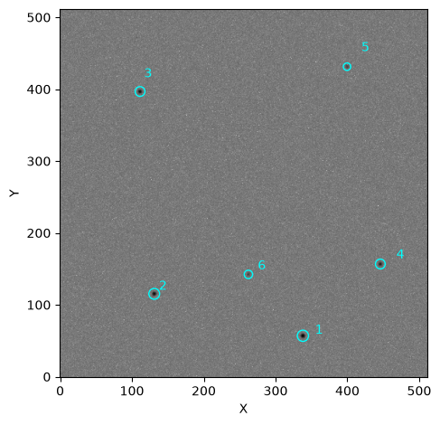
As we can see, we have once again recovered all six sources. Let’s now see how to use this custom source finder with phoptic.Reducer:
[9]:
custom_reducer = phoptic.Reducer(
    out_directory=out_dir / 'reduced' / 'custom_finder',
    data_directory=out_dir / 'data',
    finder=custom_finder,  # use custom source finder
)

custom_reducer.create_catalogs()
[OPTICAM] out/reduced/custom_finder not found, attempting to create ...
[OPTICAM] out/reduced/custom_finder created.
[OPTICAM] Scanning data directory: 100%|██████████████████████████████████████████████████████████████████████████████████████████████████████████████████████████|[00:00<00:00]
[OPTICAM] Checking instrument OPTICAM_MX.
[OPTICAM] OPTICAM_MX sucessfully passed all checks.
[OPTICAM] Parsing file headers: 100%|█████████████████████████████████████████████████████████████████████████████████████████████████████████████████████████████|[00:02<00:00]
[OPTICAM] Binning: 4x4
[OPTICAM] Filters: 1:g, 2:r, 3:i
[OPTICAM] 3 1:g images.
[OPTICAM] 3 2:r images.
[OPTICAM] 3 3:i images.
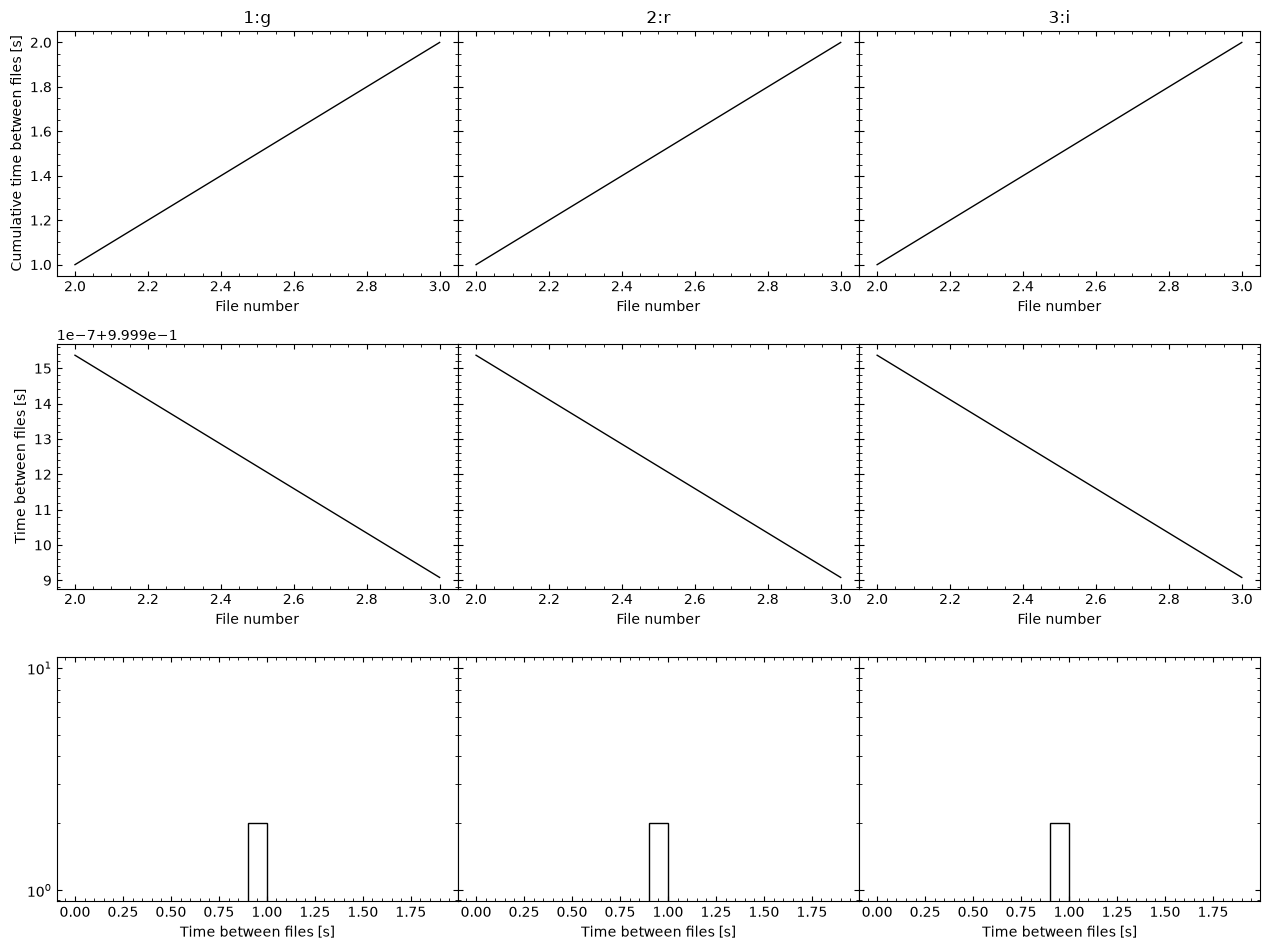
[OPTICAM] Plot saved to /tmp/tmpez9fxze7/out/reduced/custom_finder/diag/header_times.pdf.
[OPTICAM] Creating source catalogs.
[OPTICAM] Aligning 1:g images: 100%|██████████████████████████████████████████████████████████████████████████████████████████████████████████████████████████████|[00:02<00:00]
[OPTICAM] [OPTICAM] Done.
[OPTICAM] [OPTICAM] 3 image(s) aligned.
[OPTICAM] [OPTICAM] 0 image(s) could not be aligned.
[OPTICAM] Aligning 2:r images: 100%|██████████████████████████████████████████████████████████████████████████████████████████████████████████████████████████████|[00:02<00:00]
[OPTICAM] [OPTICAM] Done.
[OPTICAM] [OPTICAM] 3 image(s) aligned.
[OPTICAM] [OPTICAM] 0 image(s) could not be aligned.
[OPTICAM] Aligning 3:i images: 100%|██████████████████████████████████████████████████████████████████████████████████████████████████████████████████████████████|[00:02<00:00]
[OPTICAM] [OPTICAM] Done.
[OPTICAM] [OPTICAM] 3 image(s) aligned.
[OPTICAM] [OPTICAM] 0 image(s) could not be aligned.
[OPTICAM] Plot saved to /tmp/tmpez9fxze7/out/reduced/custom_finder/cat/catalogs.pdf.
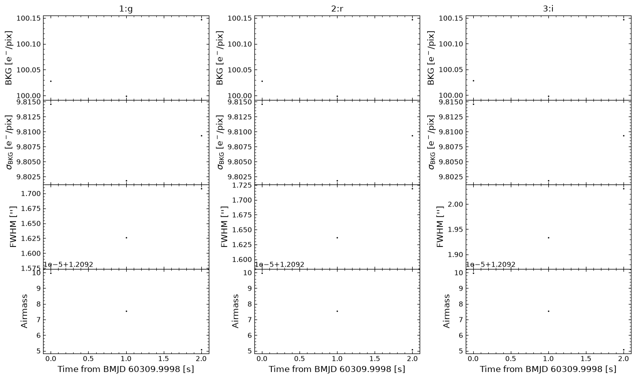
[OPTICAM] Plot saved to /tmp/tmpez9fxze7/out/reduced/custom_finder/diag/systematics.pdf.
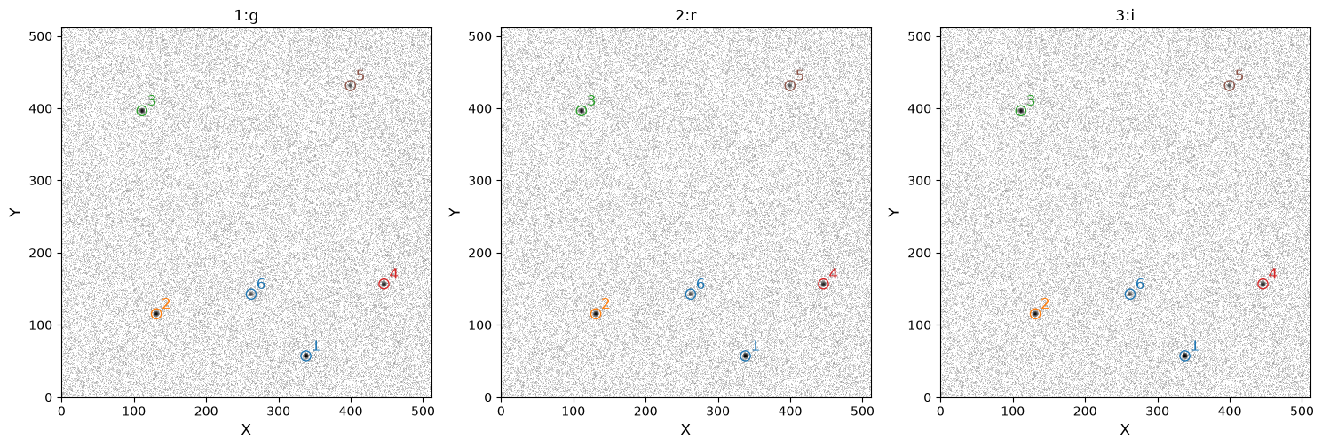
Our custom source finder has been used to successfully identify all six sources. Let’s compare this to using DefaultFinder:
[10]:
default_reducer = phoptic.Reducer(
    out_directory=out_dir / 'reduced' / 'default_finder',
    data_directory=out_dir / 'data',
)

default_reducer.create_catalogs()
[OPTICAM] out/reduced/default_finder not found, attempting to create ...
[OPTICAM] out/reduced/default_finder created.
[OPTICAM] Scanning data directory: 100%|██████████████████████████████████████████████████████████████████████████████████████████████████████████████████████████|[00:00<00:00]
[OPTICAM] Checking instrument OPTICAM_MX.
[OPTICAM] OPTICAM_MX sucessfully passed all checks.
[OPTICAM] Parsing file headers: 100%|█████████████████████████████████████████████████████████████████████████████████████████████████████████████████████████████|[00:02<00:00]
[OPTICAM] Binning: 4x4
[OPTICAM] Filters: 1:g, 2:r, 3:i
[OPTICAM] 3 1:g images.
[OPTICAM] 3 2:r images.
[OPTICAM] 3 3:i images.
[OPTICAM] Plot saved to /tmp/tmpez9fxze7/out/reduced/default_finder/diag/header_times.pdf.
[OPTICAM] Creating source catalogs.
[OPTICAM] Aligning 1:g images: 100%|██████████████████████████████████████████████████████████████████████████████████████████████████████████████████████████████|[00:02<00:00]
[OPTICAM] [OPTICAM] Done.
[OPTICAM] [OPTICAM] 3 image(s) aligned.
[OPTICAM] [OPTICAM] 0 image(s) could not be aligned.
[OPTICAM] Aligning 2:r images: 100%|██████████████████████████████████████████████████████████████████████████████████████████████████████████████████████████████|[00:02<00:00]
[OPTICAM] [OPTICAM] Done.
[OPTICAM] [OPTICAM] 3 image(s) aligned.
[OPTICAM] [OPTICAM] 0 image(s) could not be aligned.
[OPTICAM] Aligning 3:i images: 100%|██████████████████████████████████████████████████████████████████████████████████████████████████████████████████████████████|[00:02<00:00]
[OPTICAM] [OPTICAM] Done.
[OPTICAM] [OPTICAM] 3 image(s) aligned.
[OPTICAM] [OPTICAM] 0 image(s) could not be aligned.
[OPTICAM] Plot saved to /tmp/tmpez9fxze7/out/reduced/default_finder/cat/catalogs.pdf.
[OPTICAM] Plot saved to /tmp/tmpez9fxze7/out/reduced/default_finder/diag/systematics.pdf.
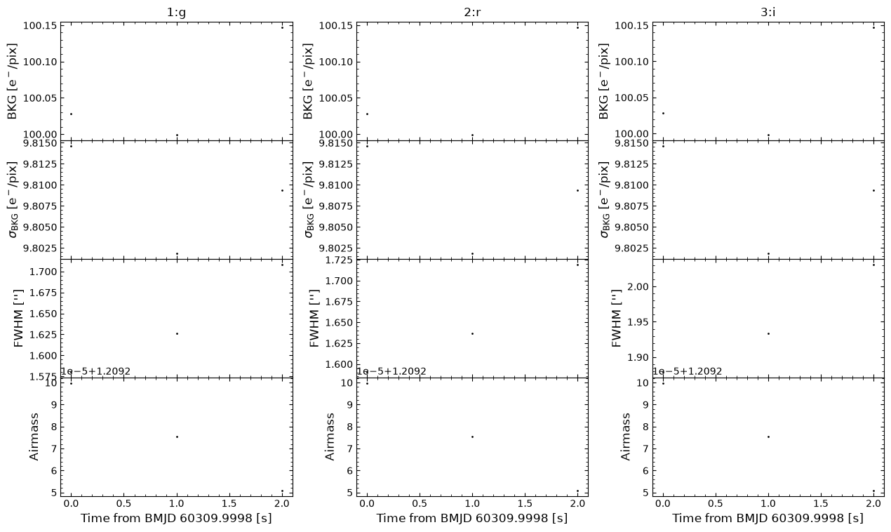
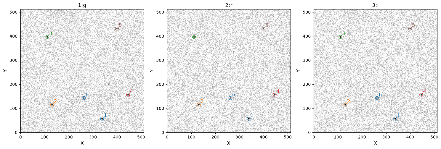
Unsurprisingly, the default source finder has also identified all six sources. Admittedly, this rather simple example does a poor job of demonstrating why defining a custom source finder may be useful, but hopefully it is clear how custom source finders can be implemented. For more information on defining custom source finders, I again refer to the excellent photutils documentation: https://photutils.readthedocs.io/en/stable/user_guide/segmentation.html. Note that phoptic requires that
source finder routines return an astropy.table.QTable instance when called, while photutils returns a SourceCatalog instance. To convert the SourceCatalog to a QTable, you can use the `to_table() <https://photutils.readthedocs.io/en/stable/api/photutils.segmentation.SourceCatalog.html#photutils.segmentation.SourceCatalog.to_table>`__ method.
That concludes the source finder tutorial for phoptic!