Timing methods

This notebook demonstrates some of the “quick-look” timing analyses available in phoptic, as well as how to extend the available timing analyses using `stingray <https://docs.stingray.science/en/stable/>`__.

Generating and Reducing Data

Before we can explore the different timing analyses provided in phoptic, we need some light curves to analyse. For this example, I’ll generate and reduce some gappy observations (see the reduction tutorial for more details on data reduction):

[1]:

import os

os.environ['OMP_NUM_THREADS'] = '1'

from pathlib import Path

import phoptic

out_dir = Path('out')

[2]:

phoptic.generate_gappy_observations(
    out_directory=out_dir / 'data',  # path to the directory where the generated data will be saved
    circular_aperture=False,  # disable circular aperture shadow
    n_images=500,
    )

[OPTICAM] variable source is at (131, 115)
[OPTICAM] variability RMS: 0.02 %
[OPTICAM] variability frequency: 0.135 Hz
[OPTICAM] variability phase lags:
    [OPTICAM] g-band: 0.000 radians
    [OPTICAM] r-band: 1.571 radians
    [OPTICAM] i-band: 3.142 radians

Generating observations: 100%|████████████████████████████████████████████████████████████████████████████████████████████████████████████████████████████████████|[00:45<00:00]

[3]:

reducer = phoptic.Reducer(
    out_directory=out_dir / 'reduced',
    data_directory=out_dir / 'data',
)

[OPTICAM] out/reduced not found, attempting to create ...
[OPTICAM] out/reduced created.

[OPTICAM] Scanning data directory: 100%|██████████████████████████████████████████████████████████████████████████████████████████████████████████████████████████|[00:00<00:00]

[OPTICAM] Checking instrument OPTICAM_MX.
[OPTICAM] OPTICAM_MX sucessfully passed all checks.

[OPTICAM] Parsing file headers: 100%|█████████████████████████████████████████████████████████████████████████████████████████████████████████████████████████████|[00:02<00:00]

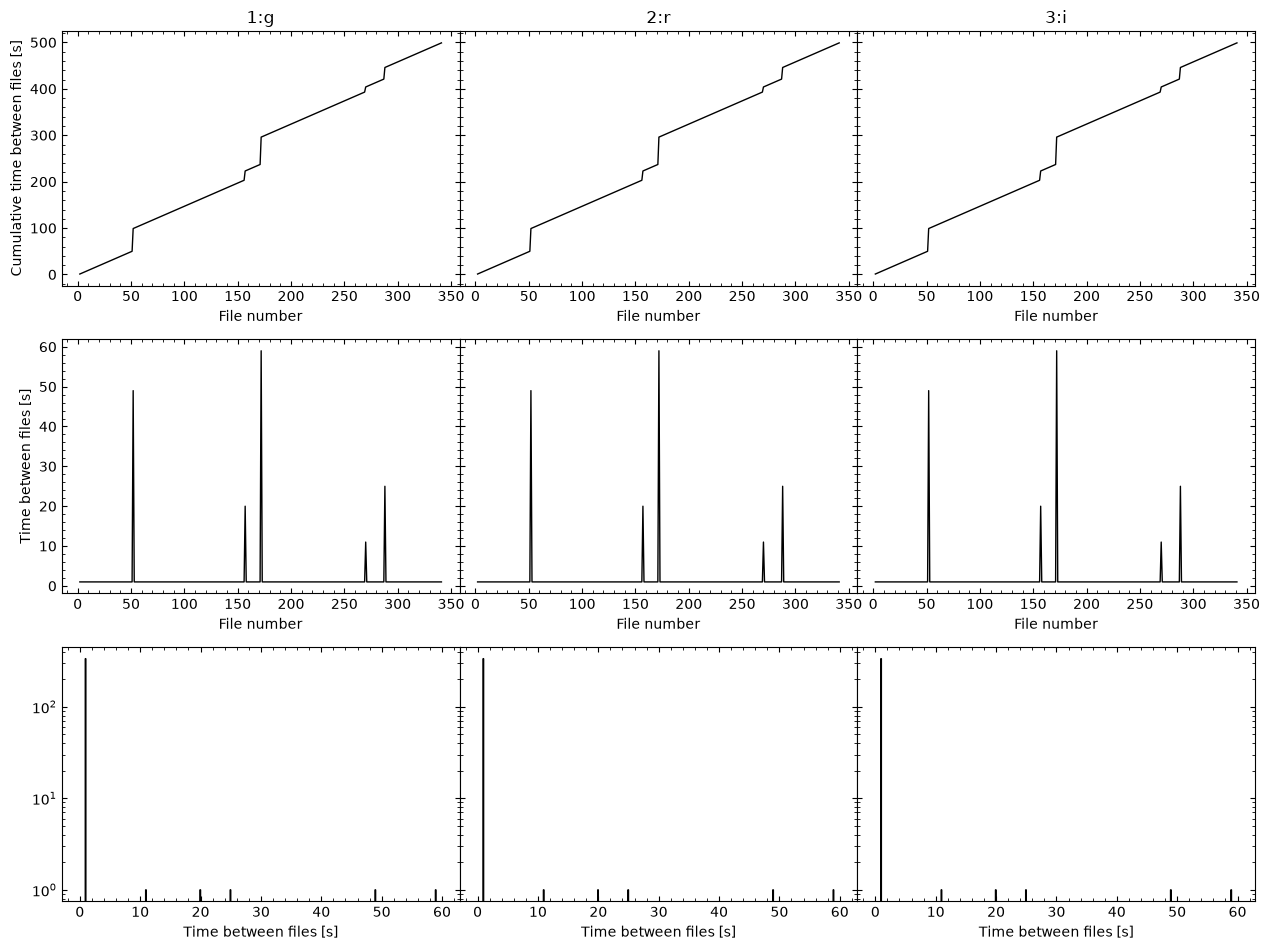
[OPTICAM] Large time gap detected between 240101r200000339o.fits and 240101g200000178o.fits (48.995 s compared to the median time difference of 1.000 s). This may cause alignment issues. If so, consider moving all files after this gap to a separate directory.
[OPTICAM] Large time gap detected between 240101g200000037o.fits and 240101r200000319o.fits (19.998 s compared to the median time difference of 1.000 s). This may cause alignment issues. If so, consider moving all files after this gap to a separate directory.
[OPTICAM] Large time gap detected between 240101r200000347o.fits and 240101g200000368o.fits (58.994 s compared to the median time difference of 1.000 s). This may cause alignment issues. If so, consider moving all files after this gap to a separate directory.
[OPTICAM] Large time gap detected between 240101i200000414o.fits and 240101r200000024o.fits (10.999 s compared to the median time difference of 1.000 s). This may cause alignment issues. If so, consider moving all files after this gap to a separate directory.
[OPTICAM] Large time gap detected between 240101r200000386o.fits and 240101r200000200o.fits (24.998 s compared to the median time difference of 1.000 s). This may cause alignment issues. If so, consider moving all files after this gap to a separate directory.
[OPTICAM] Large time gap detected between 240101r200000339o.fits and 240101g200000178o.fits (48.995 s compared to the median time difference of 1.000 s). This may cause alignment issues. If so, consider moving all files after this gap to a separate directory.
[OPTICAM] Large time gap detected between 240101g200000037o.fits and 240101r200000319o.fits (19.998 s compared to the median time difference of 1.000 s). This may cause alignment issues. If so, consider moving all files after this gap to a separate directory.
[OPTICAM] Large time gap detected between 240101r200000347o.fits and 240101g200000368o.fits (58.994 s compared to the median time difference of 1.000 s). This may cause alignment issues. If so, consider moving all files after this gap to a separate directory.
[OPTICAM] Large time gap detected between 240101i200000414o.fits and 240101r200000024o.fits (10.999 s compared to the median time difference of 1.000 s). This may cause alignment issues. If so, consider moving all files after this gap to a separate directory.
[OPTICAM] Large time gap detected between 240101r200000386o.fits and 240101r200000200o.fits (24.998 s compared to the median time difference of 1.000 s). This may cause alignment issues. If so, consider moving all files after this gap to a separate directory.
[OPTICAM] Large time gap detected between 240101r200000339o.fits and 240101g200000178o.fits (48.995 s compared to the median time difference of 1.000 s). This may cause alignment issues. If so, consider moving all files after this gap to a separate directory.
[OPTICAM] Large time gap detected between 240101g200000037o.fits and 240101r200000319o.fits (19.998 s compared to the median time difference of 1.000 s). This may cause alignment issues. If so, consider moving all files after this gap to a separate directory.
[OPTICAM] Large time gap detected between 240101r200000347o.fits and 240101g200000368o.fits (58.994 s compared to the median time difference of 1.000 s). This may cause alignment issues. If so, consider moving all files after this gap to a separate directory.
[OPTICAM] Large time gap detected between 240101i200000414o.fits and 240101r200000024o.fits (10.999 s compared to the median time difference of 1.000 s). This may cause alignment issues. If so, consider moving all files after this gap to a separate directory.
[OPTICAM] Large time gap detected between 240101r200000386o.fits and 240101r200000200o.fits (24.998 s compared to the median time difference of 1.000 s). This may cause alignment issues. If so, consider moving all files after this gap to a separate directory.
[OPTICAM] Binning: 4x4
[OPTICAM] Filters: 1:g, 2:r, 3:i
[OPTICAM] 341 1:g images.
[OPTICAM] 341 2:r images.
[OPTICAM] 341 3:i images.

/home/zac/Documents/University/PhD/Repos/opticam/phoptic/utils/data_checks.py:227: UserWarning: Large time gap detected between 240101r200000339o.fits and 240101g200000178o.fits (48.995 s compared to the median time difference of 1.000 s). This may cause alignment issues. If so, consider moving all files after this gap to a separate directory.
warnings.warn(string)
/home/zac/Documents/University/PhD/Repos/opticam/phoptic/utils/data_checks.py:227: UserWarning: Large time gap detected between 240101g200000037o.fits and 240101r200000319o.fits (19.998 s compared to the median time difference of 1.000 s). This may cause alignment issues. If so, consider moving all files after this gap to a separate directory.
warnings.warn(string)
/home/zac/Documents/University/PhD/Repos/opticam/phoptic/utils/data_checks.py:227: UserWarning: Large time gap detected between 240101r200000347o.fits and 240101g200000368o.fits (58.994 s compared to the median time difference of 1.000 s). This may cause alignment issues. If so, consider moving all files after this gap to a separate directory.
warnings.warn(string)
/home/zac/Documents/University/PhD/Repos/opticam/phoptic/utils/data_checks.py:227: UserWarning: Large time gap detected between 240101i200000414o.fits and 240101r200000024o.fits (10.999 s compared to the median time difference of 1.000 s). This may cause alignment issues. If so, consider moving all files after this gap to a separate directory.
warnings.warn(string)
/home/zac/Documents/University/PhD/Repos/opticam/phoptic/utils/data_checks.py:227: UserWarning: Large time gap detected between 240101r200000386o.fits and 240101r200000200o.fits (24.998 s compared to the median time difference of 1.000 s). This may cause alignment issues. If so, consider moving all files after this gap to a separate directory.
warnings.warn(string)

[OPTICAM] Plot saved to /tmp/tmp6mipb2u_/out/reduced/diag/header_times.pdf.

../_images/_executed_timing_methods_3_7.png

[4]:

reducer.create_catalogs()

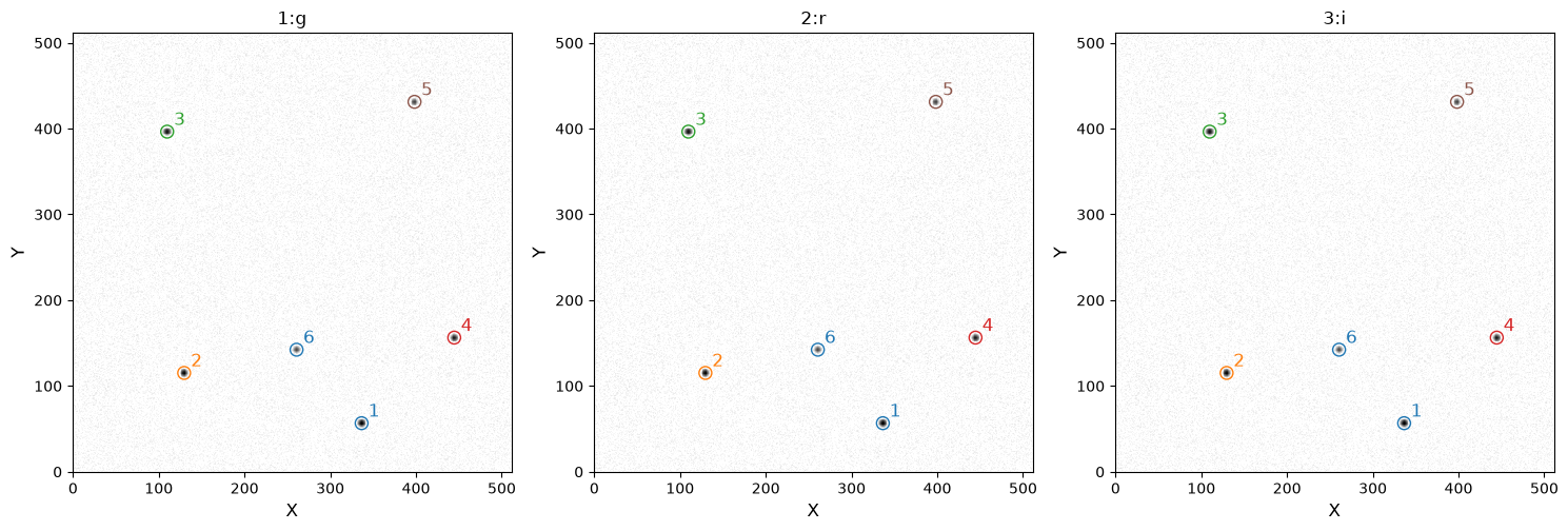
[OPTICAM] Creating source catalogs.

[OPTICAM] Aligning 1:g images: 100%|██████████████████████████████████████████████████████████████████████████████████████████████████████████████████████████████|[00:04<00:00]

[OPTICAM] [OPTICAM] Done.
[OPTICAM] [OPTICAM] 341 image(s) aligned.
[OPTICAM] [OPTICAM] 0 image(s) could not be aligned.

[OPTICAM] Aligning 2:r images: 100%|██████████████████████████████████████████████████████████████████████████████████████████████████████████████████████████████|[00:04<00:00]

[OPTICAM] [OPTICAM] Done.
[OPTICAM] [OPTICAM] 341 image(s) aligned.
[OPTICAM] [OPTICAM] 0 image(s) could not be aligned.

[OPTICAM] Aligning 3:i images: 100%|██████████████████████████████████████████████████████████████████████████████████████████████████████████████████████████████|[00:04<00:00]

[OPTICAM] [OPTICAM] Done.
[OPTICAM] [OPTICAM] 341 image(s) aligned.
[OPTICAM] [OPTICAM] 0 image(s) could not be aligned.
[OPTICAM] Plot saved to /tmp/tmp6mipb2u_/out/reduced/cat/catalogs.pdf.

../_images/_executed_timing_methods_4_7.png

[OPTICAM] Plot saved to /tmp/tmp6mipb2u_/out/reduced/diag/systematics.pdf.

../_images/_executed_timing_methods_4_9.png

[5]:

phot = phoptic.OptimalPhotometer()
reducer.photometry(phot)

[OPTICAM] [OPTICAM] Photometry results will be saved to lcs/optimal in out/reduced.

[OPTICAM] Performing photometry on 1:g images: 100%|██████████████████████████████████████████████████████████████████████████████████████████████████████████████|[00:06<00:00]
[OPTICAM] Performing photometry on 2:r images: 100%|██████████████████████████████████████████████████████████████████████████████████████████████████████████████|[00:05<00:00]
[OPTICAM] Performing photometry on 3:i images: 100%|██████████████████████████████████████████████████████████████████████████████████████████████████████████████|[00:05<00:00]

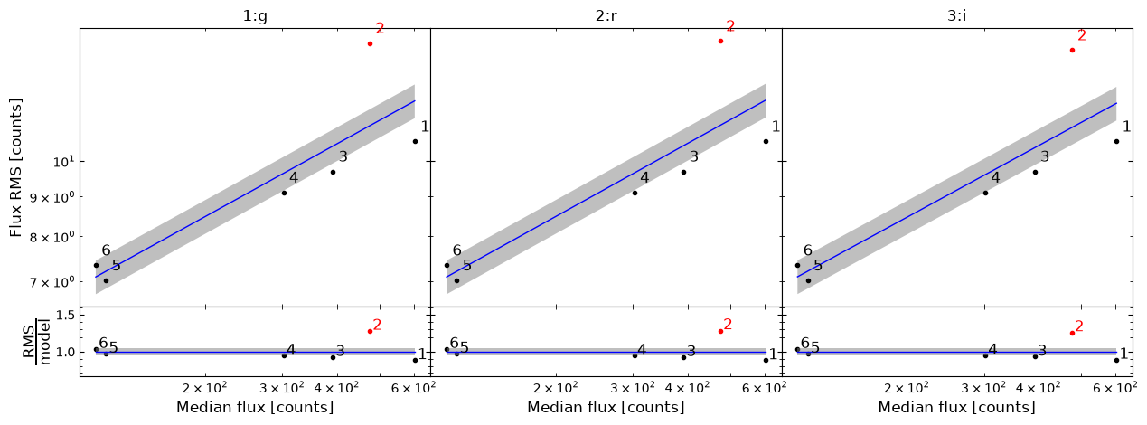
[OPTICAM] Plot saved to /tmp/tmp6mipb2u_/out/reduced/diag/optimal_rms_vs_median.pdf.

../_images/_executed_timing_methods_5_3.png

[6]:

dphot = phoptic.DifferentialPhotometer(
    out_directory=out_dir / 'reduced',
)

unnormed_analyser = dphot.get_relative_light_curve(
    key='1:g',
    target=2,
    comparisons=[1, 3, 6],
    phot_label='optimal',
    prefix='example',
    match_other_cameras=True,
    show_diagnostics=False,
)

[OPTICAM] Keys: 1:g, 2:r, 3:i

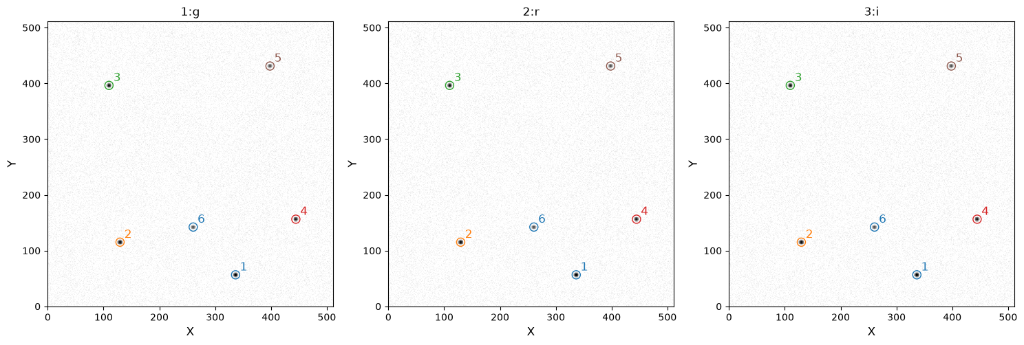
../_images/_executed_timing_methods_6_1.png

[OPTICAM] 1:g target ID 2 was matched to 2:r target ID 2
[OPTICAM] 2:r comparison ID 1 was matched to 2:r comparison ID 1
[OPTICAM] 2:r comparison ID 3 was matched to 2:r comparison ID 3
[OPTICAM] 2:r comparison ID 6 was matched to 2:r comparison ID 6
[OPTICAM] 1:g target ID 2 was matched to 3:i target ID 2
[OPTICAM] 3:i comparison ID 1 was matched to 3:i comparison ID 1
[OPTICAM] 3:i comparison ID 3 was matched to 3:i comparison ID 3
[OPTICAM] 3:i comparison ID 6 was matched to 3:i comparison ID 6

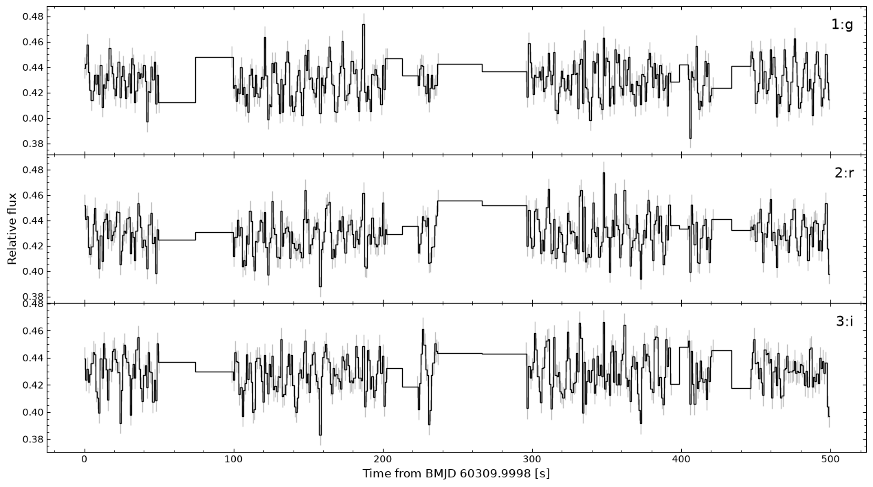
../_images/_executed_timing_methods_6_3.png

We now have an Analyzer instance that provides a number of quick-look timing analyses routines. Under-the-hood, these routines are mostly wrappers around astropy routines.

By default, light curves are not normalised when performing differential photometry. To normalise our light curves to a mean of 1, we can define a new Analyzer instance with norm='mean':

[7]:

analyser = phoptic.Analyzer(
    out_directory=out_dir / 'reduced',
    light_curves=unnormed_analyser.light_curves,
    norm='mean',
)

`phoptic.Analyzer` routines

Let’s first take a look at our Analyzer light curves using the plot() method:

[8]:

analyser.plot()

[OPTICAM] Plot saved to /tmp/tmp6mipb2u_/out/reduced/plots/None_None_light_curves.pdf.

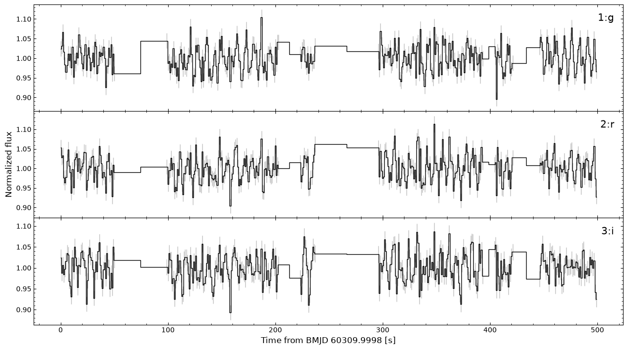
../_images/_executed_timing_methods_10_1.png

As we can see, we have three variable, gappy light curves, all with a mean flux of 1. The filter for each light curve is shown in the top right. We can also see that this figure was saved to timing_analysis_tutorial/reduced/plots/source_2_optimal_light_curves.pdf.

We can inspect our light curve data via the light_curves attribute. Within an Analyzer, light curves are stored as `astropy.timeseries.TimeSeries <https://docs.astropy.org/en/stable/timeseries/index.html>`__ instances:

We can also rebin our light curves to a lower time resolution using the rebin() method:

[9]:

from astropy import units as u

binned_analyser = analyser.rebin(time_bin_size=10 * u.s)

This method takes a time_bin_size parameter, which must be a astropy.units.Quantity, and returns a new Analyzer instance containing the binned light curves. Under-the-hood, this uses astropy’s aggregate_downsample() function, which is slow for long timeseries.

Let’s take a look at the binned light curves:

[10]:

binned_analyser.plot(save=False)

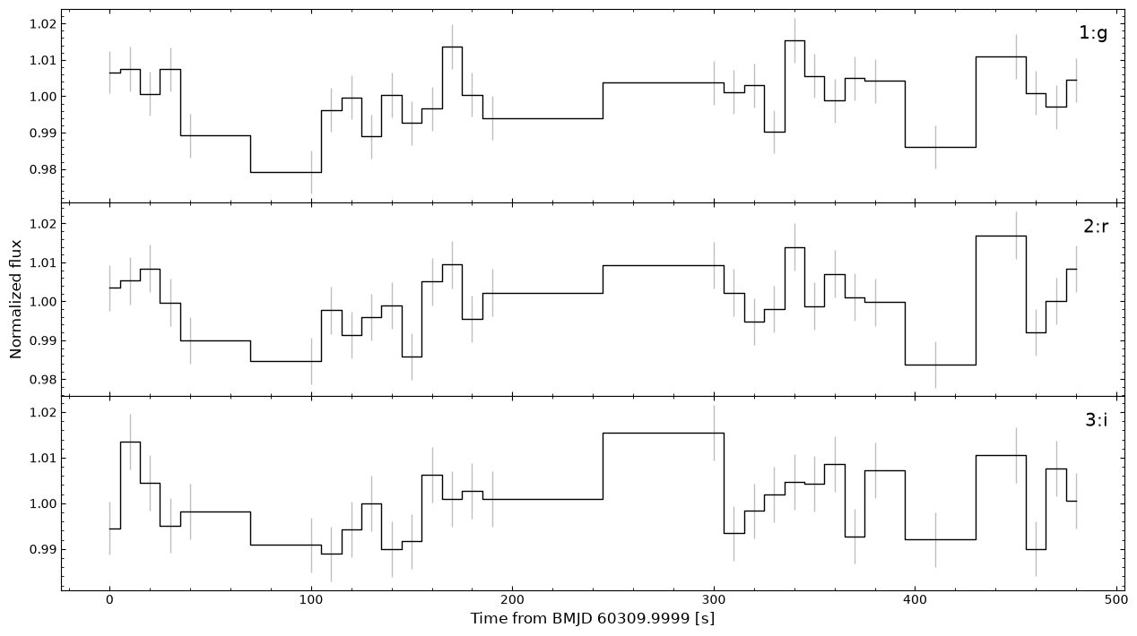
../_images/_executed_timing_methods_15_0.png

phoptic handles the error propagation during binning and avoids padding gaps in the original light curves with zeros. In this case, the bin size was too large, and the variability of the light curves has been lost. As such, we’ll carry on using the un-binned light curves.

Let’s now perform a few quick-look timing analyses on these light curves.

Lomb-Scargle Periodograms

Often times, you might want to compute the Lomb-Scargle periodograms of your light curves to check for periododic signals. astropy implements two flavours of the Lomb-Scargle periodogram: `LombScargle <https://docs.astropy.org/en/stable/timeseries/lombscargle.html>`__ and `LombScargleMultiband <https://docs.astropy.org/en/stable/timeseries/lombscarglemb.html>`__. For convenience, phoptic’s Analyzer class implements wrappers for both routines that handle the boilerplate, allowing you to get straight to the analysis.

Lomb-Scargle

Let’s first take a look at the standard Lomb-Scargle periodogram:

[11]:

lsps = analyser.lomb_scargle(scale='semilogx')

[OPTICAM] Plot saved to /tmp/tmp6mipb2u_/out/reduced/plots/None_LSP.pdf.

../_images/_executed_timing_methods_17_1.png

/home/zac/Documents/University/PhD/Repos/opticam/phoptic/analyzer.py:491: UserWarning: Attempt to set non-positive xlim on a log-scaled axis will be ignored.
  fig.clear()

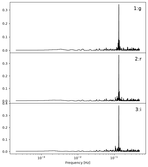
We can see that each light curve has a dedicated periodogram, and the corresponding filter is shown in the top right of each panel. In this case, all three periodograms show a sharp peak between 0.1 and 0.2 Hz.

By default, the autofrequency() method of astropy’s LombScargle class is used to construct the frequency grid of the periodogram. Alternatively, you may pass your own frequency grid. To avoid confusion with units, custom frequency grids must be passed as an astropy `Quantity <https://docs.astropy.org/en/stable/units/quantity.html>`__. For example, let’s recompute these periodograms in the 0.1-0.2 Hz frequency range. However, we do not want to overwrite our previous plot, so we’ll also pass save=False to prevent the new plot from being saved:

[12]:

from astropy import units as u
import numpy as np

frequency = np.linspace(0.1, 0.2, 100) * u.Hz  # units of Hz

lsps = analyser.lomb_scargle(frequency=frequency, save=False, scale='semilogx')

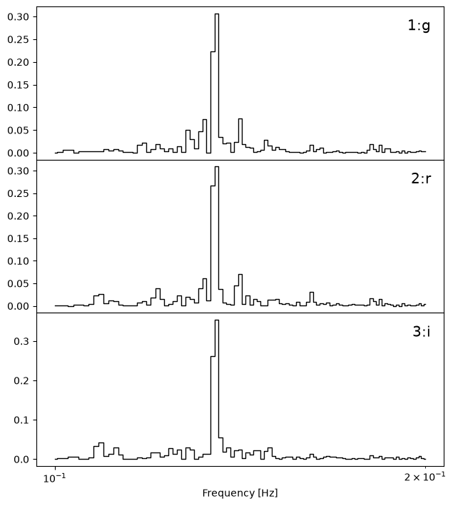
../_images/_executed_timing_methods_19_0.png

Now we can see that all three bands suggest a signal with a frequency of between 0.12 and 0.14 Hz.

Like many of the timing analysis methods of Analyzer, lomb_scargle() returns a dictionary of results that may be used to conduct further analyses. In this case, the keys list the filters and the values list the corresponding `astropy.timeseries.LombScargle <https://docs.astropy.org/en/stable/api/astropy.timeseries.LombScargle.html#astropy.timeseries.LombScargle.from_timeseries>`__ instances:

[13]:

lsps

[13]:

{'1:g': <astropy.timeseries.periodograms.lombscargle.core.LombScargle at 0x7318f980da70>,
 '2:r': <astropy.timeseries.periodograms.lombscargle.core.LombScargle at 0x7318f980d940>,
 '3:i': <astropy.timeseries.periodograms.lombscargle.core.LombScargle at 0x7318f9642450>}

Let’s use the results returned by the lomb_scargle() method to precisely infer the peak frequencies:

[14]:

import numpy as np

for fltr, lsp in lsps.items():
    power = lsp.power(frequency=frequency)
    peak_index = np.argmax(power)
    print(f'{fltr} Peak frequency = {frequency[peak_index]}')

1:g Peak frequency = 0.13535353535353536 Hz
2:r Peak frequency = 0.13535353535353536 Hz
3:i Peak frequency = 0.13535353535353536 Hz

Now we can see that all three bands show a periodicity at \(\sim\) 0.135 Hz which, as we can see at the top of this notebook, is the true frequency of variability for our source of interest.

Multiband Lomb-Scargle

In some cases, it may be preferable to compute a single Lomb-Scargle periodogram for all light curves; this can be done using astropy’s `LombScargleMultiband <https://docs.astropy.org/en/stable/timeseries/lombscarglemb.html>`__:

[15]:

periodograms = analyser.multiband_lomb_scargle(scale='semilogx')

[OPTICAM] Plot saved to /tmp/tmp6mipb2u_/out/reduced/plots/None_multiband_LSP.pdf.

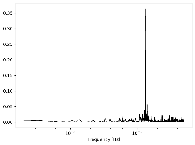
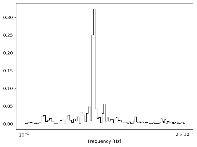
../_images/_executed_timing_methods_25_1.png

As with lomb_scargle(), custom frequency grids can also be passed to multiband_lomb_scargle():

[16]:

periodograms = analyser.multiband_lomb_scargle(frequency=frequency, save=False, scale='semilogx')

../_images/_executed_timing_methods_27_0.png

Phase Folding/Binning

Now that we have identified a candidate signal, we may want fold our light curves to see what it looks like. astropy’s TimeSeries class implements a fold() method, and phoptic’s Analyzer class provides a convenience wrapper for this method with some added functionality (binning). To fold a light curve, we need a period on which to fold; to avoid confusion with units, phoptic requires that the period being passed is a Quantity:

[17]:

f_signal = 0.135 * u.Hz  # periodogram peak frequency
p_signal = (1 / f_signal).to(u.s)  # fold period in seconds

folded_lcs = analyser.fold(
    period=p_signal,
    save=False,
)

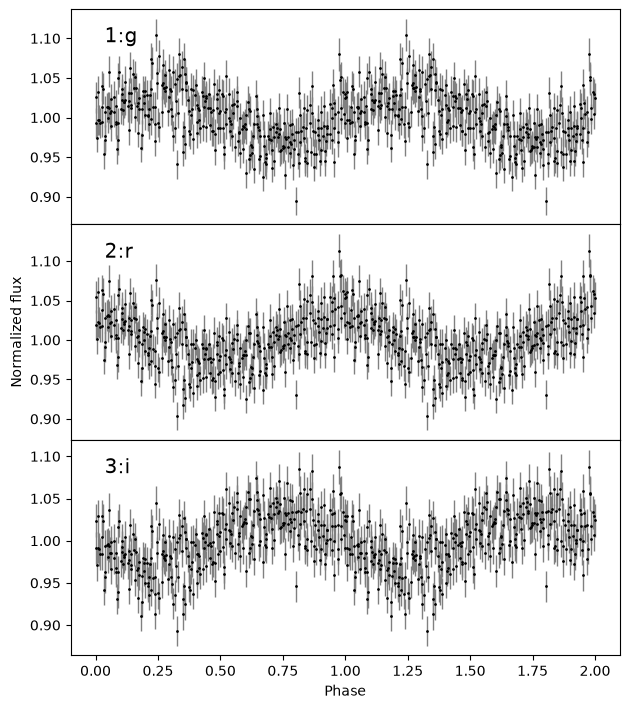
../_images/_executed_timing_methods_29_0.png

The fold() method of phoptic.Analyzer returns a TimeSeries whose "time" column quantifies the folded phase:

[18]:

folded_lcs.pprint()

       phase            1:g_rel_flux    ...   3:i_rel_flux_err
                                        ...
-------------------- ------------------ ... --------------------
-0.49985981220396775 0.9927922365231538 ... 0.018826567068287076
-0.49718195758777584 1.0254579594988855 ...  0.01942235844109346
-0.49436433950922115 0.9747686690972958 ... 0.018786333424567335
 -0.4916866546265685  1.032731595067874 ...  0.01954555786482529
 -0.4915470608977449 0.9970192309754101 ... 0.018751167112730765
-0.48605158820299826  0.996719936988276 ... 0.019086226543047577
 -0.4805560306414821 0.9927194525989773 ... 0.018785571313010306
 -0.4752006608761759 1.0138588907173431 ... 0.019236416175348534
 -0.4750604730799659 1.0399651931520213 ...  0.01930735460911876
                 ...                ... ...                  ...
 0.47252357006055423 0.9818117912596629 ... 0.018799412561319128
  0.4753411032723394 1.0796286849984926 ...  0.02045427008663402
   0.478018788154992 1.0479295012203576 ...  0.01993244061383856
  0.4808365759670859 1.0511768143222913 ... 0.019621510756137085
 0.48351417598297086 1.0114875691871112 ... 0.019339807116727895
 0.48365385457856225  0.998257350737729 ... 0.018905236996256892
  0.4918272667562702 1.0317314056470197 ...  0.01983185690004507
  0.4945047819053846   1.00469588833957 ... 0.019033371977145296
  0.4973226545842472 1.0293166050099545 ... 0.019638849865972717
  0.4999999999998224 1.0242702398309838 ... 0.019575405457908406
Length = 341 rows

Additionally, the fold() method can be used to phase bin your light curves by passing the desired number of bins to to the nbins parameter:

[19]:

folded_lcs = analyser.fold(
    period=p_signal,
    nbins=10,
    save=False,
    )

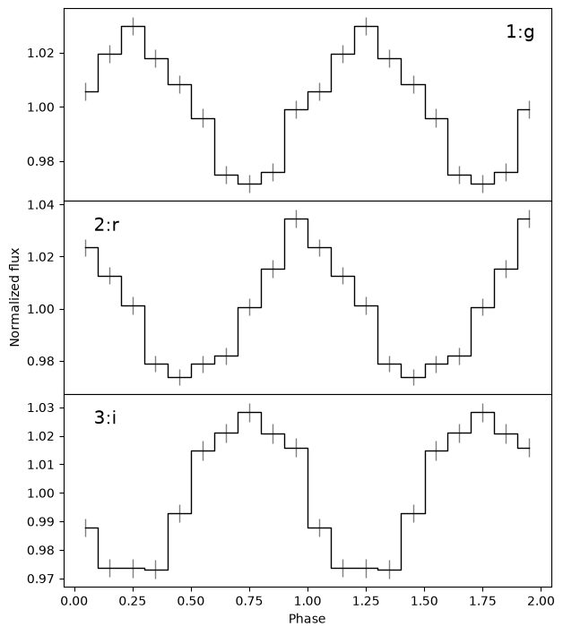
../_images/_executed_timing_methods_33_0.png

Phase binning more clearly reveals the pulse shape compared to simply folding. From the above plots, it’s clear that there is a lag in the pulsations between the different bands. Currently, phoptic does not support quantify lags natively. However, phoptic’s Analyzer class can be used to export your light curves to `stingray <https://docs.stingray.science/en/stable/>`__, which provides a much more complete timing analysis framework - including ways to compute lags. Let’s take a look at this now.

`stingray`

stingray is a feature-rich spectral timing Python package developed primarily for use with X-ray data. stingray implements a number of generic timing analyis routines that can be applied to arbitrary time series. However, since stingray was developed with X-ray data in mind, it makes certain assumptions about the data. These assumptions can cause issues for non-X-ray data, as we’ll see soon.

To export your light curves to stingray, call the export_light_curves_to_stingray() method of phoptic.Analyzer:

[20]:

stingray_lcs = analyser.export_light_curves_to_stingray()

/home/zac/miniforge3/envs/phoptic7/lib/python3.14/site-packages/stingray/utils.py:492: UserWarning: SIMON says: Stingray only uses poisson err_dist at the moment. All analysis in the light curve will assume Poisson errors. Sorry for the inconvenience.
  warnings.warn("SIMON says: {0}".format(message), **kwargs)

We can see that a warning about error distributions has been triggered. We’ll take a look at this in more detail later. For now, let’s ignore it.

export_light_curves_to_stingray() returns a dictionary of {filter: `stingray.Lightcurve <https://docs.stingray.science/en/stable/notebooks/Lightcurve/Lightcurve%20tutorial.html>`__} pairs:

[21]:

stingray_lcs

[21]:

{'1:g': <stingray.lightcurve.Lightcurve at 0x73192eab8550>,
 '2:r': <stingray.lightcurve.Lightcurve at 0x7318fa2f2850>,
 '3:i': <stingray.lightcurve.Lightcurve at 0x73192eab82d0>}

Let’s take a closer look at one of these light curves using the plot() method of stingray.Lightcurve:

[22]:

ax = stingray_lcs['1:g'].plot()

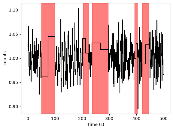
../_images/_executed_timing_methods_39_0.png

As we can see, the light curve times are converted into seconds, with \(t=0\) corresponding to the t_ref attribute of the Analyzer instance. Additionally, phoptic has automatically inferred GTIs for each light curve, which are required for compatibility with many of stingray’s methods. The shaded regions in the above plot represent the time between GTIs. Let’s use these stingray.Lightcurve instances to do some more advanced analyses.

Lags

Cross-correlation

Having recognised a lag between our light curves, there are several ways we can quantify it. For example, we can use the cross-correlations between light curves. This is a relatively simple approach, but it has the benefit of working with arbitrary time series. We can compute cross-correlations in stingray using `CrossCorrelation <https://docs.stingray.science/en/stable/notebooks/CrossCorrelation/cross_correlation_notebook.html>`__:

[23]:

from stingray.crosscorrelation import CrossCorrelation

cross_corr = CrossCorrelation(
    lc1=stingray_lcs['1:g'],
    lc2=stingray_lcs['3:i'],
    )

ax = cross_corr.plot(
    labels=['Lag [s]', 'Correlation'],
    )

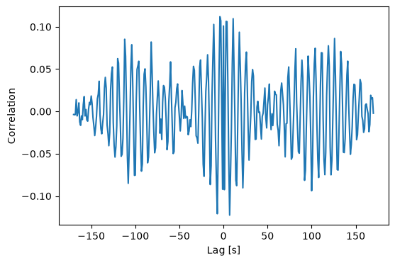
../_images/_executed_timing_methods_41_0.png

We can see that the cross-correlation spectrum peaks at a non-zero lag. We can get the exact time lag from the time_shift attribute of the CrossCorrelation instance:

[24]:

print(f'Time lag: {cross_corr.time_shift:.2f}s')

Time lag: -4.00s

We find a negative lag of about 4 s, meaning \(i\) is lagging \(g\) (as expected).

When we generated this data, we were told that the \(i\)-band variability has a phase lag of 3.142 (i.e., \(1 \pi\)) radians, while the \(g\)-band variability has a phase lag of 0 radians. We can convert this time lag into a phase lag by dividing it by the period of the variability:

[25]:

print(f'Phase lag: {2 * np.pi * cross_corr.time_shift / p_signal.to_value(u.s):.2f} radians')

Phase lag: -3.39 radians

The phase lag is a little higher than expected, but this is due to the time resolution of our light curves.

Cross-correlating generally works well, provided the light curves are dominated by the signal of interest. In many cases, however, light curves show variability on many time-scales, and we may want to isolate the lags of signals at specific frequencies. In such cases, it may be preferable to compute the cross-spectrum.

Cross-spectra

A Cautionary Tale

To compute cross-spectra, we can use stingray’s AveragedCrossspectrum class:

[26]:

from stingray import AveragedCrossspectrum
from matplotlib import pyplot as plt

segment_size = 30 * u.s

avg_cs = AveragedCrossspectrum.from_lightcurve(
    lc1=stingray_lcs['1:g'],
    lc2=stingray_lcs['3:i'],
    norm='frac',
    segment_size=segment_size.to_value(u.s),  # stingray assumes all time values are in seconds
)

avg_cs_amplitude = np.abs(avg_cs.power)

fig, ax = plt.subplots(tight_layout=True)

ax.step(
    avg_cs.freq,  # convert freq from cyc/d to Hz
    avg_cs_amplitude,
    where='mid',
    c='k',
)

ax.set_xlabel('Frequency [Hz]')
ax.set_ylabel('Power [(frac. rms)$^2$ / Hz]')

plt.show()

8it [00:00, 18396.07it/s]
/home/zac/miniforge3/envs/phoptic7/lib/python3.14/site-packages/stingray/fourier.py:1766: UserWarning: n_ave is below 30. Please note that the error bars on the quantities derived from the cross spectrum are only reliable for a large number of averaged powers.
  warnings.warn(
/home/zac/miniforge3/envs/phoptic7/lib/python3.14/site-packages/stingray/fourier.py:1800: RuntimeWarning: invalid value encountered in sqrt
  dphi = np.sqrt((1 - gsq) / (2 * gsq * n_ave))

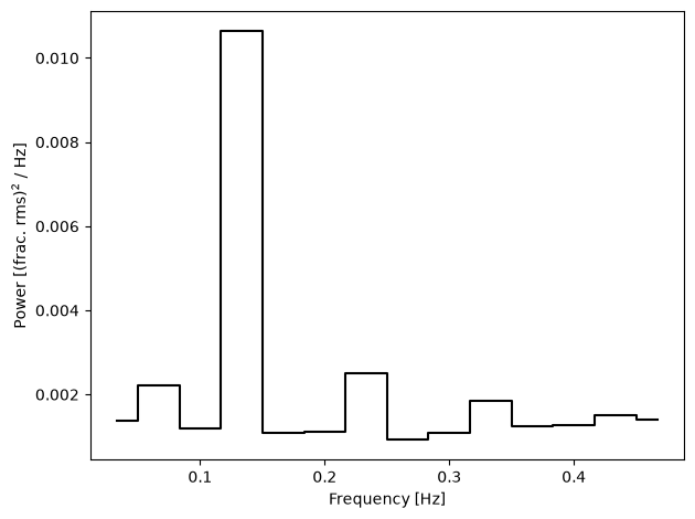
../_images/_executed_timing_methods_47_1.png

As we can see, the cross spectrum amplitude looks similar to the Lomb-Scargle periodograms we saw earlier, which is what we would expect. So far so good. Let’s try to compute the coherence between these two light curves and check it’s in the expected range (\(0 \leq \text{coherence} \leq 1\)):

[27]:

coh, coh_err = avg_cs.coherence()

print(np.logical_and(coh >= 0, coh <= 1).all())

False

/home/zac/miniforge3/envs/phoptic7/lib/python3.14/site-packages/stingray/utils.py:492: UserWarning: SIMON says: Number of segments used in averaging is significantly low. The result might not follow the expected statistical distributions.
  warnings.warn("SIMON says: {0}".format(message), **kwargs)

Uh oh, we have unphysical coherence values! Let’s take a look at some of them:

[28]:

for i in range(5):
    print(f'Coherence: {coh[i]}, error: {coh_err[i]}')

Coherence: 262213.4203728212, error: 0.125
Coherence: 100564.33319550438, error: 0.125
Coherence: 319021.37505371566, error: 0.125
Coherence: 2710.173065650526, error: 0.125
Coherence: 368492.96124993864, error: 0.125

Our coherence estimates are in the thousands, and our error estimates in the negative thousands. Something is very wrong…

The issue is due to stingray assuming Poisson statistics. Since we know the phase lag between these two light curves, let’s see what happens if we try to compute it from the averaged cross spectrum:

[29]:

plags, plags_err = avg_cs.phase_lag()

fig, ax = plt.subplots(tight_layout=True)

ax.errorbar(
    avg_cs.freq,
    plags,
    plags_err,
    fmt='kx',
)

ax.axvline(
    0.135,
    c='red',
    label='Lag frequency'
    )
ax.axhline(
    np.pi,
    c='blue',
    label='Expected lag'
    )
ax.legend()

ax.set_xlabel('Frequency [Hz]')
ax.set_ylabel('Phase lag [rad]')

plt.show()

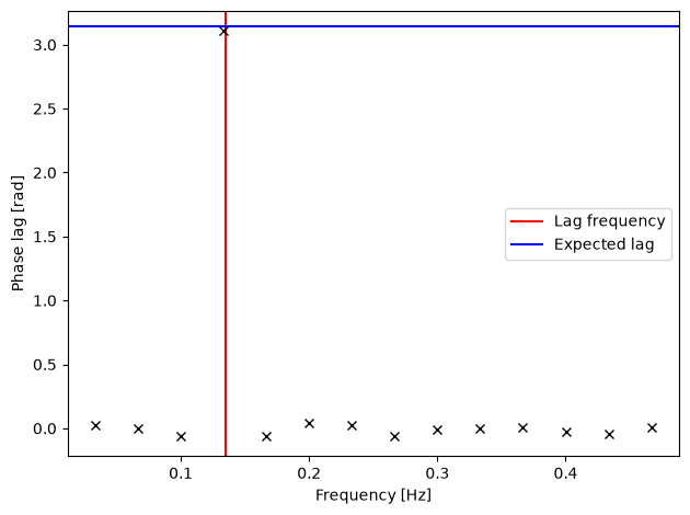
../_images/_executed_timing_methods_53_0.png

We get the correct phase lag at the correct frequency. However, we don’t seem to have any error bars, and so it’s impossible to quantify the significance of this lag. Let’s see what our error bars are:

[30]:

print(plags_err)

[nan nan nan nan nan nan nan nan nan nan nan nan nan nan]

Our errors are all NaNs! This is another consequence of our light curves not being Poissonian. For cross spectral analyses, stingray may therefore not be suitable. For power spectra, however, stingray can be used without issue provided a suitable normalisation is specified (e.g., norm="frac").

That concludes the timing methods tutorial for phoptic! The timing methods of Analyzer demonstrated here are intended as “quick-look” analyses, while more complete analyses are made easy thanks to stingray. Note, however, that stingray may not always work as intended when applied to relative light curves.